This is a long overdue article, my apologies.
The basis of the article surrounds a question in the comments section of an article on Chandoo.org (comment #75) written about the hyperlink() method I discovered and wrote about here. In Chandoo’s example, when a user rolls over different “hotspots” representing different datasets, the corresponding data comes into view on a graph below. In other words, the rollover technique tells Excel to change the data currently being fed into the chart. One of the respondents to his post attempted an associated technique that would create a dynamic hyperlink to the dataset. The goal, essentially, was to create an “edit” button that could bring the user to the dataset in view.
The problem he (and I) ran into was that whenever we updated the link in the Hyperlink formula, the hyperlink's friendly name, “Edit,” would be replaced by the address of the actual link. This resulted in an Edit hyperlink that read something like “Sheet!A1” instead of “Edit Sales.” While the link worked, the result was ugly. We needed to try something different.
So here's my solution. It’s nothing really fancy, but it does require you to keep track of two components: (1) the tab that holds your associated data; and (2) the beginning cell of your associated data. There are, indeed, many ways to keep track of this information, but some planning and organization helps out a lot. One of the easiest organization techniques is to have your data in the same cell for each tab. If your “Sales” data begins in cell B1, then any other data you'd like to use for this technique should also start in B1. Moreover, if you're interested in information from your sales tab, name your tab “Sales” (and your other tabs “expenses,” “income,” etc.). Similarly, if you are pulling from different databases, tab one could be Database1, tab two Databse2, etc. Alas, not all data can be organized in this manner, but you get the picture. Such organization makes a significant difference when implementing this technique and my example below assumes you have data from tabs Database1, Database2, and Database3.

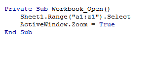
For example, when the user places his or her mouse of cell B5, C5, or D5 the following code is executed.
Hopefully this is all review for you. If not – or, for a quick refresher – read these:
1. Rollover b8 ov1
2. Interactive Dashboard in Excel using Hyperlinks
On to the Good Stuff
So now we need a button that, when clicked, will take us to the location where the data resides. As you might have noticed from my example above, I placed a textbox on my dashboard with the label “Edit.” This is my edit “hyperlink.” But instead of actually “hyperlinking” to the data, I’ll instead tell Excel to take me to the data with a macro. In my module I’ve written the following code and have assigned it to the textbox.
Here’s what’s going on. In the earlier code section – my ChangeSelection function – I told excel to change the named range, valSelOption, to an index representing the location where my data resides. But I’ve also named my tabs Database1, Database2, and Database3. Since I placed my data starting in range B2 for each tab, I can use valSelOption to direct Excel to the correct tab. In the above code, I create a worksheet object and assign it to the correct worksheet by concatenating “Database” with valSelOption. In other words, if I valSelOption is 1, then the database we want will be Database1...and so forth.
Also, notice that my code first activates the tab we want before activating the range within it. This is an important step that must come first or you will surely get an error.
---
So what if your data isn't organized in an easy, uniform way? Well, in my example, you might change cells B3 to D3 to the name of your tabs. And in your ChangeSelection() function you would have a string argument instead of an integer. That could help your program identify the tab housing your data. Again there are different ways to do this.
But if you find that your data is all over the place – consider reorganizing!
-
(I’ll have the file up with this example soon.)
The basis of the article surrounds a question in the comments section of an article on Chandoo.org (comment #75) written about the hyperlink() method I discovered and wrote about here. In Chandoo’s example, when a user rolls over different “hotspots” representing different datasets, the corresponding data comes into view on a graph below. In other words, the rollover technique tells Excel to change the data currently being fed into the chart. One of the respondents to his post attempted an associated technique that would create a dynamic hyperlink to the dataset. The goal, essentially, was to create an “edit” button that could bring the user to the dataset in view.
The problem he (and I) ran into was that whenever we updated the link in the Hyperlink formula, the hyperlink's friendly name, “Edit,” would be replaced by the address of the actual link. This resulted in an Edit hyperlink that read something like “Sheet!A1” instead of “Edit Sales.” While the link worked, the result was ugly. We needed to try something different.
So here's my solution. It’s nothing really fancy, but it does require you to keep track of two components: (1) the tab that holds your associated data; and (2) the beginning cell of your associated data. There are, indeed, many ways to keep track of this information, but some planning and organization helps out a lot. One of the easiest organization techniques is to have your data in the same cell for each tab. If your “Sales” data begins in cell B1, then any other data you'd like to use for this technique should also start in B1. Moreover, if you're interested in information from your sales tab, name your tab “Sales” (and your other tabs “expenses,” “income,” etc.). Similarly, if you are pulling from different databases, tab one could be Database1, tab two Databse2, etc. Alas, not all data can be organized in this manner, but you get the picture. Such organization makes a significant difference when implementing this technique and my example below assumes you have data from tabs Database1, Database2, and Database3.
A Quick Refresher

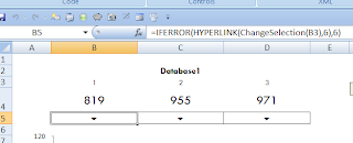
The dashboard above works the same way as the example used in Chandoos’ post. The cell’s with the down arrows are the rollover hotspots and they contain the required hyperlink formulas.

For example, when the user places his or her mouse of cell B5, C5, or D5 the following code is executed.
Public Function ChangeSelection(i As Integer)

     Range("valSelOption") = i

End Function
Hopefully this is all review for you. If not – or, for a quick refresher – read these:
1. Rollover b8 ov1
2. Interactive Dashboard in Excel using Hyperlinks
On to the Good Stuff
So now we need a button that, when clicked, will take us to the location where the data resides. As you might have noticed from my example above, I placed a textbox on my dashboard with the label “Edit.” This is my edit “hyperlink.” But instead of actually “hyperlinking” to the data, I’ll instead tell Excel to take me to the data with a macro. In my module I’ve written the following code and have assigned it to the textbox.
Public Sub GoToData()
Dim wsCurrent As Excel.Worksheet
Set wsCurrent = Worksheets("Database" & Range("valSelOption"))
wsCurrent.Activate
wsCurrent.Range("B2").Activate
End Sub
Here’s what’s going on. In the earlier code section – my ChangeSelection function – I told excel to change the named range, valSelOption, to an index representing the location where my data resides. But I’ve also named my tabs Database1, Database2, and Database3. Since I placed my data starting in range B2 for each tab, I can use valSelOption to direct Excel to the correct tab. In the above code, I create a worksheet object and assign it to the correct worksheet by concatenating “Database” with valSelOption. In other words, if I valSelOption is 1, then the database we want will be Database1...and so forth.
Also, notice that my code first activates the tab we want before activating the range within it. This is an important step that must come first or you will surely get an error.
---
So what if your data isn't organized in an easy, uniform way? Well, in my example, you might change cells B3 to D3 to the name of your tabs. And in your ChangeSelection() function you would have a string argument instead of an integer. That could help your program identify the tab housing your data. Again there are different ways to do this.
But if you find that your data is all over the place – consider reorganizing!
-
(I’ll have the file up with this example soon.)